
For pathfinding and collision avoidance, many methods have been proposed. In this article, I would like to share a classical approach, graphic search, which is very interesting and has been applied in many fields. This article will introduce the family and braches of graph search and give an insight into how it works in collision avoidance.
The most straightforward graph search algorithm is Breadth-First Search [1]. It simply checks all the possibilities from near and far until the first solution is found. As a brute-force algorithm, Breadth-First Search is simple but with typically low computational efficiency.
One well-known pathfinding algorithm was proposed by a Dutch programmer Edsger Dijkstra in 1956 [2], and named after him, which can be regarded as one of the earliest artificial intelligence (AI) methods, with another name, uniform cost search. It aims to find the shortest path between points a and b. Its execution process is simple: i) starting from the current point a, ii) calculating the cost/distance to all neighbors, iii) choosing the neighbor with minimum accumulated cost/distance, iv) starting from the current point and repeating until reaching the destination. Of course, the same point can be reached from different neighbors, but usually with different accumulated costs. We only choose the path with a smaller cost/distance. A typical graphic map is illustrated in Figure 1.
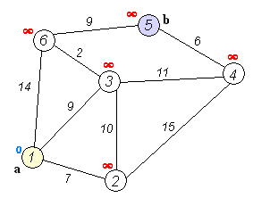
Figure 1: Finding the best path from a to b on a graphic map [3]
Compared to the Breadth-First Search which explores equally in all directions, Dijkstra’s Algorithm favors lower-cost paths. However, Dijkstra’s algorithm explores the map without any directional information, even if we already know a general direction that we want to go. For example, let’s image that we are in a forest and want to leave it. And now we see a signal showing the exit of the forest. Unfortunately, Dijkstra’s algorithm does not use this information. What can we do if we want to use this signal information? The straightforward idea is to move directly to the signal position regardless of other factors, which is Greedy Best First Search . We are following the default rule that the shortest distance between our current position and the signal is always prioritized. Of course, you can do that, but probably you have to cross rivers and climb over the mountains. Besides, what if the signal’s position is not exactly the position of the exit? Intuitively, a better way can be to use the signal as a reference to guide us while still using Dijkstra’s algorithm to explore the lower-cost path first. That is precisely how A* looks like.

Figure 2: Expansion demonstrations of different algorithms (some subfigures refer to Amit Patel [4])
Dijkstra’s algorithm works well to find the shortest path, but it wastes time exploring directions that aren’t promising. Greedy Best First Search explores promising directions, but it may not find the shortest path. The A* algorithm uses both the actual distance from the start and the estimated distance to the goal. The total cost function,  , of A* consists of historical exact cost and heuristic cost:

Where  represents the exact cost of the path from the starting point to any point
  , and
, and  represents the heuristic estimated cost from any point to the destination.
The proposition of A* inspired people with a new way for such pathfinding problems. Countless variants have been constantly proposed. The original A* defaults that the historic and heuristic components equally impact the search progress. However, that might not be the fact. Thus, one idea is to add weight factors to the two components, such as weighted A* and dynamic weighted A* [5][6]. From the following equation with weight factors, we can find the relationship between these algorithms:
 or
or 
When the heuristic weight is higher, A* will search more toward the destination. In the situation that ,  ,
,  , then A* is the same as Greedy Best First Search. On the contrary, when ,
  ,
,  , A* becomes Dijkstra’s algorithm. From a computational speed point of view, Dijkstra’s algorithm is slow but ensures the best solution, while the greedy search is fast but non-optimal. Thus, finding the proper weight factors becomes a problem in balancing the computational effectiveness and efficiency. More variants were proposed to ensure the computational speed with sufficient computational effectiveness, e.g., the bidirectional search and jump point search.
So far, the problem description is all about pathfinding, which is simple. However, in practice, usually, the map is dynamic, the environment is unknown, and the vehicle you are driving/controlling is underactuated. All these factors make it a complex collision avoidance case. Let’s take the maritime sailing scenario as an example. Our ship can meet multiple other vessels from different directions. And the map constraints can contain not only geometry limit (shore), but also the water depth and restricted areas. To solve all these practical problems, more variants have been proposed. Dynamic A* or D* was proposed to cope with changing environment [7]. Lifelong Planning A* and D* lite were further proposed using less search effort [8]. In order to cope with the motion constraints from the vehicle, one variant, Hybrid A* was proposed [9], that associates a continuous state with each cell. Another way is to modify the path with an additional path smoothing post-processing step taking the dynamic or kinematic into account. Furthermore, we also proposed a Hybrid A* based method with a floating-node map associated with the discretized control setpoints [10].
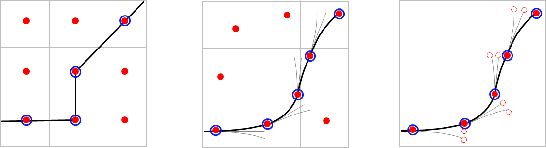
Figure 3: Graphical comparison of search algorithms. Left: A* only visits grid center. Center: Hybrid A* associates a continuous state with each cell, so it can visit all the positions within a cell. Right: improved Hybrid A* searches in a node map. [10]
In addition, although it is called the graph search algorithm, it can also be used in other places. The a and b in Figure 1 can be the ‘state points’ in a system. For instance, if you are parking a car, you want to move your car from the current position onto the parking space. You can give different control actions, e.g., controlling the throttle or turning the wheel, and you know the consequence of each action. Regardless of other aspects, let’s say you want to finish the parking as soon as possible. You can set the time as an optimization goal. So graph search algorithms can be used to find the best action paths (combinations) to park the car. Of course, in practice, getting a cost map for each action is not easy. Here we only want to show the feasibility of using this graphic search method for different tasks.
Figure 4: A parking scenario
References
[1] Lee, C.Y., 1961. An algorithm for path connections and its applications. IRE transactions on electronic computers, (3), pp.346-365.[2] Dijkstra, E.W., 1959. A note on two problems in connexion with graphs. Numerische mathematik, 1(1), pp.269-271.
[3] Wikipedia Contributors (2019). Dijkstra’s algorithm. [online] Wikipedia. Available at: https://en.wikipedia.org/wiki/Dijkstra%27s_algorithm.
[4] Redblobgames.com. (2014). Red Blob Games: Introduction to A*. [online] Available at: https://www.redblobgames.com/pathfinding/a-star/introduction.html.
[5] Pohl, I. (1970). Heuristic search viewed as path finding in a graph. Artificial Intelligence, 1(3-4), pp.193–204. doi:10.1016/0004-3702(70)90007-x.
[6] Chen, J. and Sturtevant, N.R., 2021, May. Necessary and Sufficient Conditions for Avoiding Reopenings in Best First Suboptimal Search with General Bounding Functions. In AAAI Conference on Artificial Intelligence.
[7] Stentz, A., 1997. Optimal and efficient path planning for partially known environments. In Intelligent unmanned ground vehicles (pp. 203-220). Springer, Boston, MA.
[8] Koenig, S., Likhachev, M. and Furcy, D. (2004). Lifelong Planning A∗. Artificial Intelligence, 155(1-2), pp.93–146. doi:10.1016/j.artint.2003.12.001.
[9] Dolgov, D., Thrun, S., Montemerlo, M. and Diebel, J., 2008. Practical search techniques in path planning for autonomous driving. Ann Arbor, 1001(48105), pp.18-80.
[10] Miao, T., El Amam, E., Slaets, P. and Pissoort, D., 2022. An improved real-time collision-avoidance algorithm based on Hybrid A* in a multi-object-encountering scenario for autonomous surface vessels. Ocean Engineering, 255, p.111406.
About the Author: Tianlei Miao
 Tianlei has studied in Naval Architecture and Ocean Engineering at Zhejiang University, where he graduated with his bachelor’s degree in 2017. During his bachelor’s years, Tianlei was awarded several scholarships such as National Scholarship in China and has held different leadership positions, such as President of the Student Union of Ocean College at Zhejiang University. He also spent 6 months at the Technical University of Munich in Mechanical Engineering.
In 2017, Tianlei started a dual M.Sc in Maritime Engineering at both Norwegian University of Science and Technology (NTNU), Norway, and the Royal Institute of Technology (KTH), Sweden. As part of the master’s program, he focused on the generation of the full-envelope hydrodynamic database of hydrostatic AUVs under the supervision of Prof. Dr. Ivan Stenius and Prof.Dr. Marilena Greco.
![]()